---
title: "TidyTuesday: Long Beach Animal Shelter"
description: ""
author:
- name: Jess Graves
date: 03-01-2025
execute-dir: project
crossref:
fig-title: '**Figure**'
tbl-title: '**Table**'
fig-labels: arabic
tbl-labels: arabic
title-delim: "."
link-citations: true
execute:
echo: true
warning: false
message: false
categories: [tidy tuesday, data visualization] # self-defined categories
image: preview-image.png
draft: false
# bibliography: references.bib
nocite: |
@*
# csl: statistics-in-biosciences.csl
bibliographystyle: apa
citation: true
---
# This week's dataset (2025-03-04)
This week's tidytuesday included a published dataset from Long Beach Animal Shelter. Here's what their [README](https://github.com/rfordatascience/tidytuesday/tree/main/data/2025/2025-03-04) says:
::: {.callout-note appearance="minimal"}
This week we're exploring the [Long Beach Animal Shelter Data](https://data.longbeach.gov/explore/dataset/animal-shelter-intakes-and-outcomes/information/)!
The dataset comes from the [City of Long Beach Animal Care Services](https://www.longbeach.gov/acs/) via the [{animalshelter}](https://emilhvitfeldt.github.io/animalshelter/) R package.
> This dataset comprises of the intake and outcome record from Long Beach Animal Shelter.
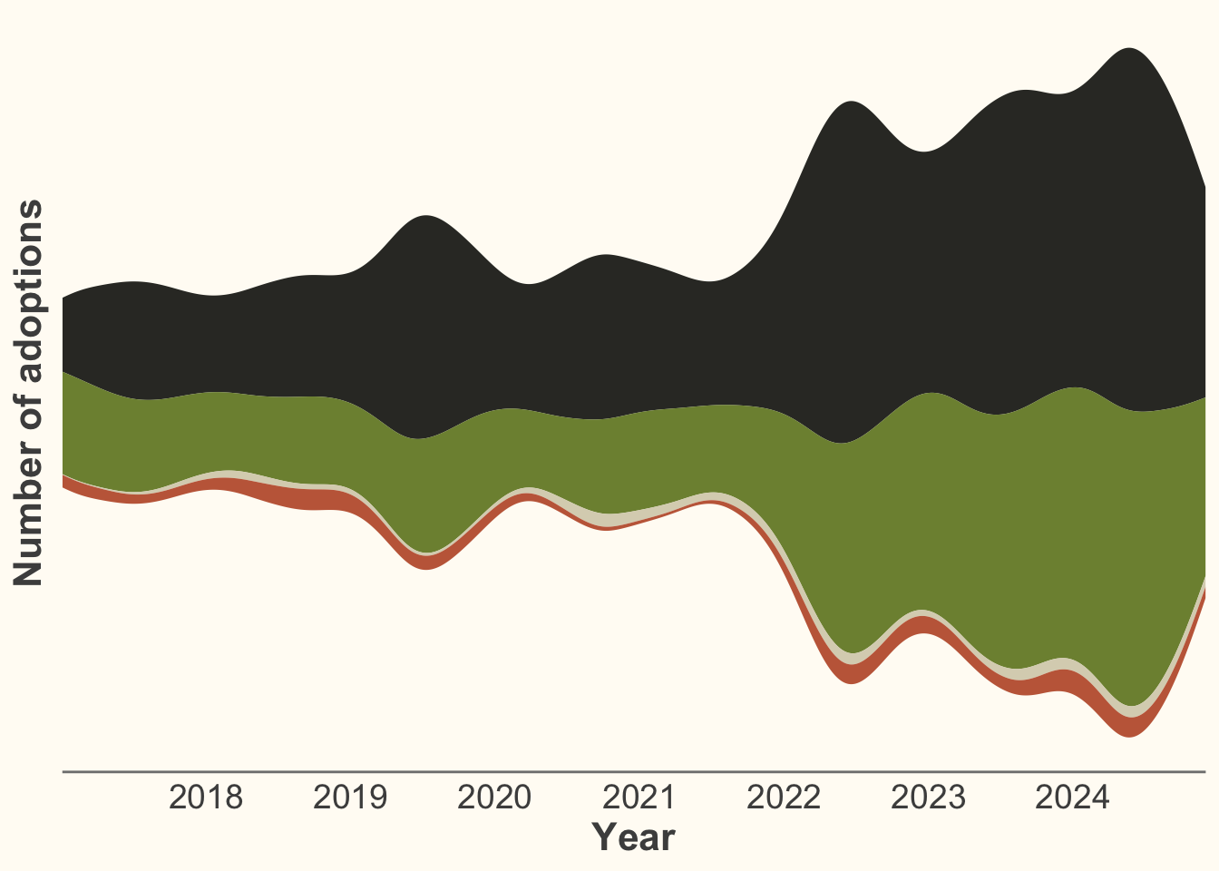
- How has the number of pet adoptions changed over the years?
- Which type of pets are adopted most often?
:::
## What I hope to visualize
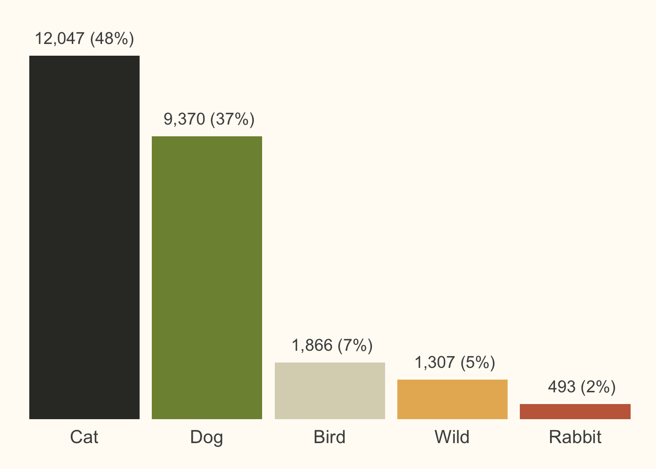
- What pets are represented in the dataset?
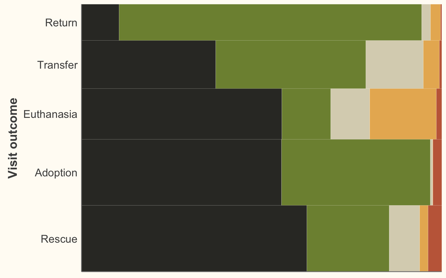
- What outcomes are most likely to occur in different pets?
- Have visit rates changed over time?
# Data
```{r}
#| code-summary: Libraries
library(tidyverse)
library(styler)
library(patchwork)
library(ggmosaic)
library(colorspace)
library(paletteer)
library(ggstream)
library(gtsummary)

# c1 <- "#FDFBE4FF"
c2 <- lighten("#FFFBF2", amount = 0.3)

choice <- c2
# setting ggplot theme
my_theme <- theme_classic() +
  theme(
    axis.title = element_text(size = 16, color = "grey30",
                              face = "bold"),
    axis.text = element_text(size = 14, color = "grey30"),
    axis.line = element_line(color = "grey50"),
    strip.text = element_text(size = 14),
    plot.background = element_rect(
      color =  choice,
      fill = choice
    ),
    panel.background = element_rect(
      color = choice,
      fill = choice
    )
  )

palette <- "lisa::FridaKahlo"
alpha = 0.9

theme_set(my_theme)
today <- Sys.Date()

longbeach <- readr::read_csv('https://raw.githubusercontent.com/rfordatascience/tidytuesday/main/data/2025/2025-03-04/longbeach.csv')
```
```{r}
#| code-summary: Tabulating animal types and outcome types
longbeach %>%
  dplyr::select(animal_type, outcome_type)  %>%
  tbl_summary()
```
There seem to be some redundant outcome types, so I am going to combine a few categories
```{r}
#| code-fold: false
longbeach <- longbeach %>%
  filter(animal_type !='other',
         outcome_type != 'duplicate')  %>%
  mutate(age = difftime(intake_date, dob, units='days')/365.25,
         outcome_type_clean = case_when(grepl('neuter', outcome_type) ~ 'neuter',
                                        grepl('return', outcome_type) ~ 'return',
                                        grepl('foster', outcome_type) ~ 'foster',
                                        grepl('disposal', outcome_type) ~ 'died',
                                        TRUE ~ outcome_type )) %>%
  mutate(across(c(outcome_type_clean, animal_type), str_to_sentence))
```
For the sake of de-cluttering, I'm only going to look at the top 5 most frequent pets and top 5 most frequent outcome types.
```{r}
#| code-summary: Top 5 most frequent pets and outcomes
animal_levels <- longbeach %>%
  group_by(animal_type) %>%
  tally() %>%
  arrange(desc(n)) %>%
  slice(1:5)

outcome_levels <-longbeach %>%
  group_by(outcome_type_clean) %>%
  tally() %>%
  arrange(desc(n)) %>%
  slice(1:5)
```
# Most frequent visits & outcome types
```{r}
data_clean <- longbeach %>%
  filter(animal_type %in% animal_levels$animal_type,
         outcome_type_clean %in% outcome_levels$outcome_type_clean) %>%
  mutate(animal_type = factor(animal_type,
                              levels = animal_levels$animal_type),
         outcome_type_clean = factor(outcome_type_clean,
                              levels = outcome_levels$outcome_type_clean),
         )
```
```{r}
#| fig-height: 5
#| fig-width: 8
p_mosaic <- data_clean %>%
  ggplot() +
  geom_mosaic(aes(x=product(outcome_type_clean),
                  fill=animal_type),
              offset=0.001, alpha=alpha)+
  theme(legend.position ='none',
        axis.text.x= element_blank(),
        axis.ticks = element_blank(),
        axis.title.x = element_blank(),
        axis.title.y = element_text(margin=margin(r=5,
                                                  l=5))) +
  scale_x_productlist(expand=c(0, 0)) +
  scale_y_productlist(expand=c(0, 0)) +
  coord_flip() +
  labs(y='Pet', x='Visit outcome') +
  scale_fill_paletteer_d(palette)
p_mosaic
```
```{r}
p_hist <- data_clean %>%
  group_by(animal_type) %>%
  tally() %>%
  mutate(percent = paste0(round(100*n/sum(n), 0), '%'),
         n_pct = paste0(format(n, big.mark = ','), ' (', percent, ')')) %>%
  ggplot(aes(x=animal_type, y=n, fill=animal_type)) +
  geom_bar(stat='identity',
           alpha=alpha) +
  scale_fill_paletteer_d(palette) +
  guides(fill = 'none') +
  geom_text(aes(label = n_pct, y = n),
            vjust = -1,
            color = 'grey30',
            size=4.5) +
  theme(axis.line = element_blank(),
        axis.text.y = element_blank(),
        axis.title = element_blank(),
        axis.ticks = element_blank(),
        axis.text.x = element_text(vjust=5),
        plot.title = element_text(size=18, color = 'grey30',
                                  hjust=1)) +
  scale_y_continuous(limits = c(0, 13000))
p_hist
```
# Number of adoptions over time
```{r}
p_stream <- data_clean %>%
  filter(outcome_type_clean == 'Adoption') %>%
  mutate(year_mo = floor_date(intake_date, "month")) %>%
  group_by(year_mo, animal_type) %>%
  tally() %>%
  mutate(animal_type = factor(animal_type, levels = animal_levels$animal_type)) %>%
  ggplot(aes(x=year_mo,
             y = n,
             fill=animal_type)) +
  geom_stream(alpha=alpha) +
  scale_fill_paletteer_d(palette, drop = FALSE) +
  scale_x_date(date_breaks = "1 year",
               date_labels = '%Y',
               expand = c(0, 0)) +
  theme(axis.text.y=element_blank(),
        axis.ticks=element_blank(),
        axis.line.y=element_blank()) +
  labs(x='Year', y='Number of adoptions') +
  guides(fill = FALSE)
p_stream
```
# Combining
## Version 1
```{r}
#| fig-width: 10
#| fig-height: 10
p_bottom <- (p_hist + plot_spacer() + p_mosaic + theme(axis.title.y=element_blank())) +
    plot_layout(nrow = 1, widths = c(2, 0.1, 1))
(p_stream / p_bottom )+
  plot_layout(nrow=2,
              heights = c(1, 0.5))
```
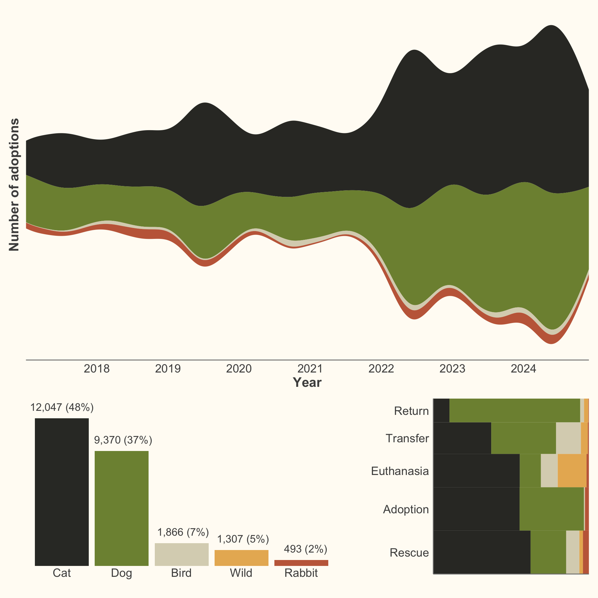
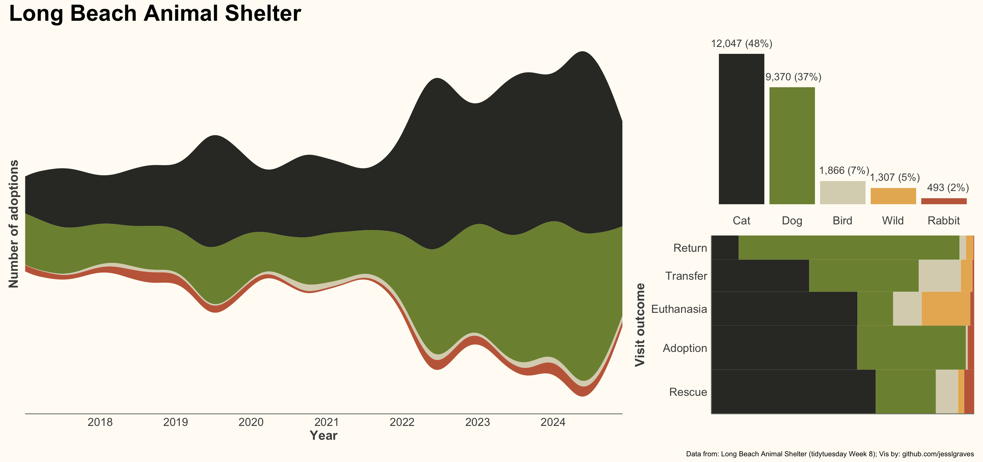
## Version 2 (Final version)
```{r}
right_side <- (p_hist +
    theme(axis.text.x = element_text(vjust=1))) /
  (p_mosaic) +
  plot_layout(ncol = 1,
              heights = c(1, 1))
```
```{r}
#| fig-width: 17
#| fig-height: 8
final <- (p_stream | right_side) + plot_layout(widths = c(2.5, 1.1))+
  plot_annotation(title = 'Long Beach Animal Shelter',
                  caption = 'Data from: Long Beach Animal Shelter (tidytuesday Week 8); Vis by: github.com/jesslgraves') &
  theme(plot.title = element_text(size=28, face = 'bold'))

final
ggsave('preview-image.png', final,
       units='cm',
       width = 50,
       height = 25)
```