“There has been increasing debate around how or if race and ethnicity should be used in medical research—including the conceptualization of race as a biological entity, a social construct, or a proxy for racism. The objectives of this narrative review are to identify and synthesize reported racial and ethnic inequalities in obstetrics and gynecology (ob/gyn) and develop informed recommendations for racial and ethnic inequity research in ob/gyn.”
What I hope to visualize
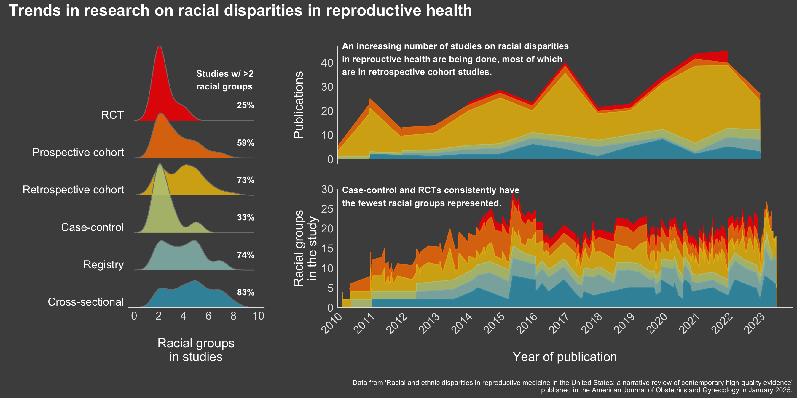
We know already that science has historically failed to enroll representative groups. And so, with this data I wanted to explore two things:
Are there differences in representation in racial groups across study types – that is, are we more likely to get better representation in cohort studies or clinical trials?
Are there changes in the magnitude of representation over time – have we seen improvements in cohort representatives over the years?
article_dat <-read_csv('data/article_dat.csv') %>%# combining month, day, year into date datamutate(date =make_date(year, month, day), # calculate total number of groups representedn_races =rowSums(!is.na(select(., c(contains('race'), -contains('_ss')))), na.rm =TRUE), # n_ethnicity = rowSums(!is.na(select(., c(contains('eth'), # -contains('_ss')))), # na.rm = TRUE), # cleaning sudy type datastudy_type =factor(if_else(study_type=='RCT', study_type, str_to_sentence(study_type)), levels =c('Cross-sectional', 'Registry', 'Case-control', 'Retrospective cohort', 'Prospective cohort', 'RCT'))) %>%# dropping any without study data or no race informationfilter(!is.na(study_type), n_races >0)# setting color palette based on number of study typesstudy_pal <-wes_palette(name='Zissou1', n=length(unique(article_dat$study_type)), type='continuous')
fig <- (p1 | (p2/p3)) +plot_annotation(title ="Trends in research on racial disparities in reproductive health",caption ="\nData from 'Racial and ethnic disparities in reproductive medicine in the United States: a narrative review of contemporary high-quality evidence'\npublished in the American Journal of Obstetrics and Gynecology in January 2025.",theme =list(plot.title =element_text(size =20, face ="bold", color ="white"),plot.caption =element_text(color ="white") ) ) +plot_layout(widths =c(0.75, 2.5) )
Making some labels to annotate the text – I recently learned about inset_element() from the {patchwork} library – nice for adding text to a already patchworked figure.
Making annotations for plot
label1 <-ggplot() +annotate("text", x =1, y =5,size=4,fontface ='bold',label ="Studies w/ >2\nracial groups", hjust=0,color ='white', ) +coord_cartesian(clip ="off") +theme_void()label2 <-ggplot() +annotate("text", x =1, y =5,size=4,fontface ='bold',label ="An increasing number of studies on racial disparities\nin reprouctive health are being done, most of which\nare in retrospective cohort studies.", hjust=0,color ='white', ) +coord_cartesian(clip ="off") +theme_void()label3 <-ggplot() +annotate("text", x =1, y =5,size=4,fontface ='bold',label ="Case-control and RCTs consistently have\nthe fewest racial groups represented.", hjust=0,color ='white', ) +coord_cartesian(clip ="off") +theme_void()# adding labelsfinal_fig <- fig +inset_element(label1,left =-0.31,top =0.87,bottom =0.87,right =-0.31) +inset_element(label2, left =0.01, top =1, bottom =0.9, right =0.01) +inset_element(label3, left =0.01, top =0.45, bottom =0.4, right =0.01)
Code
final_fig
Citation
BibTeX citation:
@online{graves2025,
  author = {Graves, Jess},
  title = {TidyTuesday: {Racial} Disparities in Reproductive Research},
  date = {2025-02-26},
  url = {https://JessLGraves.github.io/posts/2025-02-26-tidytuesday/},
  langid = {en}
}
---title: "TidyTuesday: Racial disparities in reproductive research"description: ""author: - name: Jess Gravesdate: 02-26-2025execute-dir: projectcrossref: fig-title: '**Figure**' tbl-title: '**Table**' fig-labels: arabic tbl-labels: arabic title-delim: "."link-citations: trueexecute: echo: true warning: false message: falsecategories: [tidy tuesday, data visualization] # self-defined categoriesimage: preview-image.pngdraft: false # bibliography: references.bibnocite: | @*# csl: statistics-in-biosciences.cslbibliographystyle: apacitation: true---# This week's dataset (2025-02-25)This week's tidytuesday included a published dataset from review article [Racial and ethnic disparities in reproductive medicine in the United States: a narrative review of contemporary high-quality evidence](https://www.ajog.org/article/S0002-9378(24)00775-0/fulltext) published in the *American Journal of Obstetrics and Gynecology* in January 2025. Here's what their [README](https://github.com/rfordatascience/tidytuesday/tree/main/data/2025/2025-02-25) says:::: {.callout-note appearance="minimal"}This week we're exploring data on studies investigating racial and ethnic disparities in reproductive medicine as published in the eight highest impact peer-reviewed Ob/Gyn journals from January 1, 2010 through June 30, 2023. The data were collected as part of a review article [Racial and ethnic disparities in reproductive medicine in the United States: a narrative review of contemporary high-quality evidence](https://www.ajog.org/article/S0002-9378(24)00775-0/fulltext) published in the *American Journal of Obstetrics and Gynecology* in January 2025.> "There has been increasing debate around how or if race and ethnicity should be used in medical research—including the conceptualization of race as a biological entity, a social construct, or a proxy for racism. The objectives of this narrative review are to identify and synthesize reported racial and ethnic inequalities in obstetrics and gynecology (ob/gyn) and develop informed recommendations for racial and ethnic inequity research in ob/gyn.":::## What I hope to visualizeWe know already that science has historically failed to enroll representative groups. And so, with this data I wanted to explore two things:- Are there differences in representation in racial groups across study types – that is, are we more likely to get better representation in cohort studies or clinical trials?- Are there changes in the magnitude of representation over time – have we seen improvements in cohort representatives over the years?# Data```{r}#| code-summary: Libraries library(tidytuesdayR)library(tidyverse)library(renv)library(styler)library(ggridges)library(colorspace)library(wesanderson)library(patchwork)# setting ggplot thememy_theme <-theme_classic() +theme(axis.title =element_text(size =16, color ="white"),axis.text =element_text(size =14, color ="grey90"),axis.line =element_line(color ="grey90"),strip.text =element_text(size =14),plot.background =element_rect(color ="grey30",fill ="grey30" ),panel.background =element_rect(color ="grey30",fill ="grey30" ) )theme_set(my_theme)``````{r}#| code-summary: Downloading and saving data locally#| include: false# data <- tidytuesdayR::tt_load('2025-02-25')# write_csv(data$article_dat, 'data/article_dat.csv')# write_csv(data$model_dat, 'data/model_dat.csv')``````{r}#| code-summary: Reading in dataset & cleaningarticle_dat <-read_csv('data/article_dat.csv') %>%# combining month, day, year into date datamutate(date =make_date(year, month, day), # calculate total number of groups representedn_races =rowSums(!is.na(select(., c(contains('race'), -contains('_ss')))), na.rm =TRUE), # n_ethnicity = rowSums(!is.na(select(., c(contains('eth'), # -contains('_ss')))), # na.rm = TRUE), # cleaning sudy type datastudy_type =factor(if_else(study_type=='RCT', study_type, str_to_sentence(study_type)), levels =c('Cross-sectional', 'Registry', 'Case-control', 'Retrospective cohort', 'Prospective cohort', 'RCT'))) %>%# dropping any without study data or no race informationfilter(!is.na(study_type), n_races >0)# setting color palette based on number of study typesstudy_pal <-wes_palette(name='Zissou1', n=length(unique(article_dat$study_type)), type='continuous')``````{r}#| code-summary: Quick glance at dataarticle_dat %>% dplyr::select(date, contains("race")) %>%head()```# Making panels for figureI'm going to be using:- `geom_density_ridges()` from the {[`ggridges`](https://cran.r-project.org/web/packages/ggridges/vignettes/introduction.html)} library to visualize the distribution of representation across study types- `geom_area()` from the {[`ggplot2`](https://ggplot2.tidyverse.org/reference/geom_ribbon.html)} library to visualizes changes in numbers of publications and representation over time and study types```{r}#| code-summary: Panel 1 figure # setting ridge overlapridge_overlap <-2p1 <- article_dat %>%ggplot(aes(x=n_races, y=study_type, fill=study_type)) +geom_density_ridges(alpha=0.9, scale=ridge_overlap, color ='grey50') +scale_fill_manual(values=study_pal) +labs(y='', x='Racial groups\nin studies') +theme(legend.position ='none',axis.line.y =element_blank(), axis.ticks =element_blank(), axis.text.y =element_text(vjust=-0.25, color ="white") )+scale_x_continuous(breaks=seq(0, 10, by=2), limits=c(0, 10), expand=c(0, 0.5)) +scale_y_discrete(expand =c(0.00, 0))# Calculating % that have > 2 racial groups in their studiessum_dat <- article_dat %>%group_by(study_type) %>%summarize(n_more_2=sum(n_races >2), total =n(), pct=paste0(round(100*n_more_2/total), '%')) %>%mutate(x=rep(9, times=6))# adding to figure p1 <- p1 +geom_text(data=sum_dat, mapping =aes(x=x, y=study_type, label = pct), inherit.aes=F, color ='white', vjust=-2, fontface ='bold' )``````{r}#| code-summary: Panel 2 figurep2 <- article_dat %>%group_by(study_type, year) %>%tally() %>%mutate(year_mo =make_date(year), study_type =factor(study_type, levels =rev(levels(article_dat$study_type)))) %>%ggplot(aes(x=year_mo, y = n, fill = study_type, color = study_type)) +geom_area(alpha =0.9, position ="stack") +theme(legend.position ="none",axis.text.x =element_blank(),axis.line.x =element_blank(),axis.title.x=element_blank(),strip.placement ="outside",axis.ticks =element_blank(),plot.margin =margin(1, 0, 0, 0.5, "cm") ) +labs(x ="\nYear of publication", y ="\nPublications",color ="", fill ="" ) +scale_fill_manual(values =rev(study_pal)) +scale_color_manual(values =rev(study_pal)) +scale_x_date(date_breaks ="1 years",date_labels ="%Y",expand =c(0, 0),limits =c(as.Date("2010-01-01"),as.Date("2023-12-31") ) ) +guides(fill =guide_legend(ncol =3))``````{r}#| code-summary: Panel 3 figurep3 <- article_dat %>%mutate(study_type =factor(study_type, levels =rev(levels(article_dat$study_type)))) %>%ggplot(aes(x = date,y = n_races,fill = study_type, color = study_type, )) +geom_area(alpha =0.9, position ="stack") +theme(legend.position ="none",axis.text.x =element_text(angle =45, hjust =1),strip.placement ="outside",axis.ticks =element_blank(),plot.margin =margin(1, 0, 0, 0.5, "cm") ) +labs(x ="\nYear of publication", y ="\nRacial groups\nin the study",color ="", fill ="" ) +scale_fill_manual(values =rev(study_pal)) +scale_color_manual(values =rev(study_pal)) +scale_y_continuous(breaks =seq(0, 30, by =5),expand =c(0, 0),limits =c(0, 30) ) +scale_x_date(date_breaks ="1 years",date_labels ="%Y",expand =c(0, 0),limits =c(as.Date("2010-01-01"),as.Date("2023-12-31") ) ) +guides(fill =guide_legend(ncol =3))```# Combining for final figureLibrary {[`patchwork`](https://patchwork.data-imaginist.com)} comes in handy here!```{r}fig <- (p1 | (p2/p3)) +plot_annotation(title ="Trends in research on racial disparities in reproductive health",caption ="\nData from 'Racial and ethnic disparities in reproductive medicine in the United States: a narrative review of contemporary high-quality evidence'\npublished in the American Journal of Obstetrics and Gynecology in January 2025.",theme =list(plot.title =element_text(size =20, face ="bold", color ="white"),plot.caption =element_text(color ="white") ) ) +plot_layout(widths =c(0.75, 2.5) )```Making some labels to annotate the text – I recently learned about `inset_element()` from the {patchwork} library – nice for adding text to a already patchworked figure.```{r}#| code-summary: Making annotations for plotlabel1 <-ggplot() +annotate("text", x =1, y =5,size=4,fontface ='bold',label ="Studies w/ >2\nracial groups", hjust=0,color ='white', ) +coord_cartesian(clip ="off") +theme_void()label2 <-ggplot() +annotate("text", x =1, y =5,size=4,fontface ='bold',label ="An increasing number of studies on racial disparities\nin reprouctive health are being done, most of which\nare in retrospective cohort studies.", hjust=0,color ='white', ) +coord_cartesian(clip ="off") +theme_void()label3 <-ggplot() +annotate("text", x =1, y =5,size=4,fontface ='bold',label ="Case-control and RCTs consistently have\nthe fewest racial groups represented.", hjust=0,color ='white', ) +coord_cartesian(clip ="off") +theme_void()# adding labelsfinal_fig <- fig +inset_element(label1,left =-0.31,top =0.87,bottom =0.87,right =-0.31) +inset_element(label2, left =0.01, top =1, bottom =0.9, right =0.01) +inset_element(label3, left =0.01, top =0.45, bottom =0.4, right =0.01) ``````{r}#| fig-width: 14#| fig-height: 7final_fig``````{r}#| include: falsefinal_fig %>%ggsave('preview-image.png', ., units='cm',width =35, height =20)```