Figure 2. Boom! One line! geom_stream, you’re so easy!
Alright, going to try to make it a little more aesthetically pleasing, but using {colorspace} to choose my color palette. Because the Franchises are ordered by earliest release date, I’m going to go with a sequential color palette.
Code for setting palette
n_franchise <-length(unique(df$Franchise))# Palette for streamspal <-sequential_hcl(n_franchise, "BluGrn")# Palette for labelspal2 <-darken(sequential_hcl(n_franchise, "BluGrn"), amount =0.2, space ="HCL")
Code for color palette figure
color_data <-tibble(color =factor(seq_along(pal)),value =1)color_data %>%ggplot(aes(x = color, y = value, fill = color)) +geom_bar(stat ="identity") +scale_fill_manual(values = pal) +theme(legend.position ="none",axis.ticks =element_blank(),axis.text =element_blank(),axis.line =element_blank(),plot.title =element_text(hjust =0.5) ) +labs(x ="", y ="", title ="My custom palette")
Figure 3. Checking out what my palette will look like
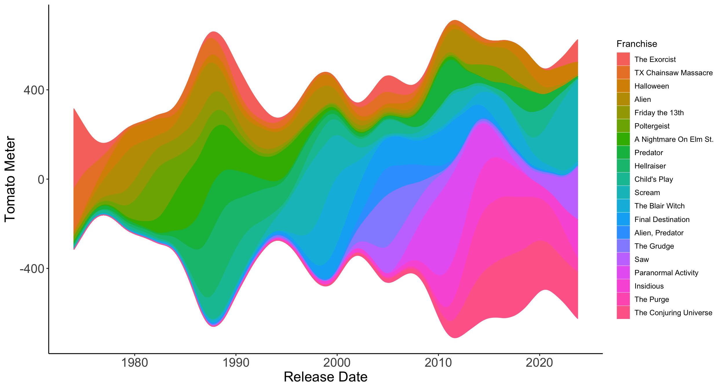
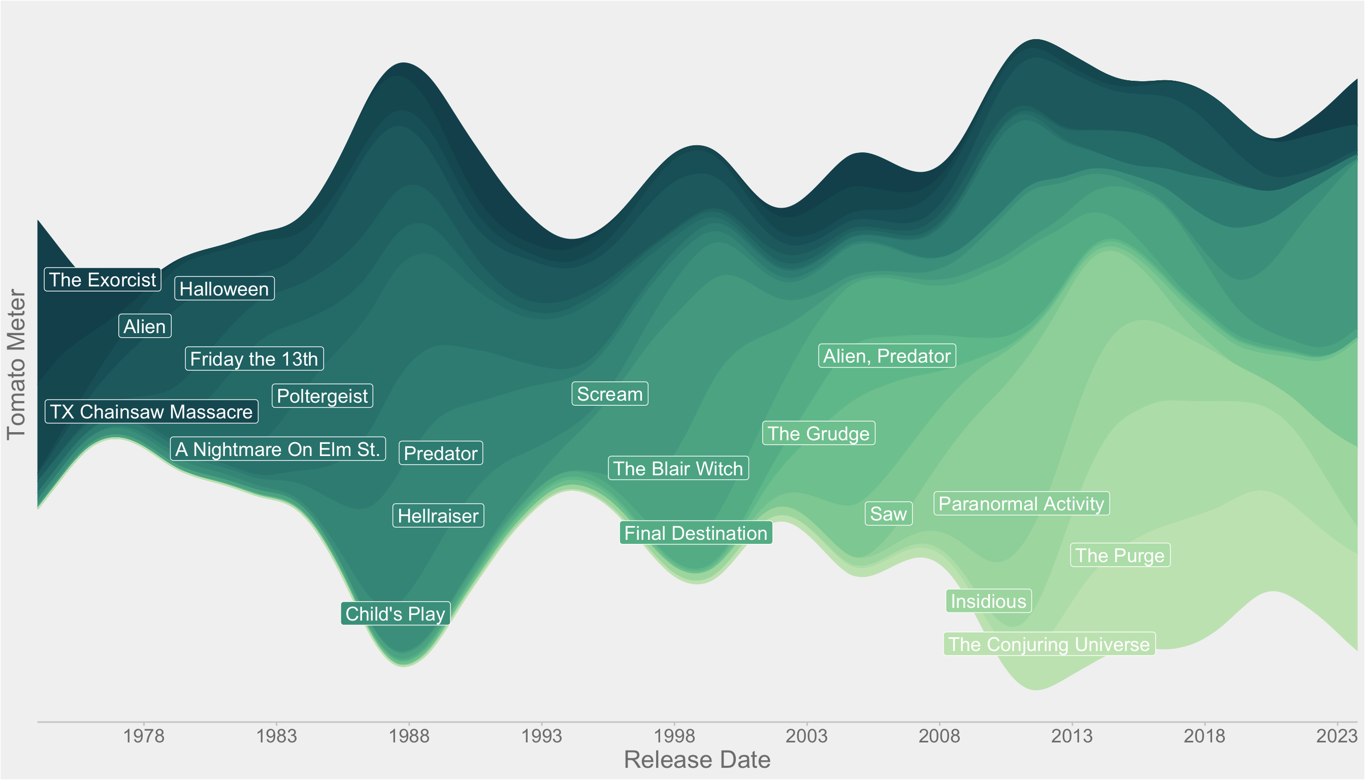
Figure 4. Tomatometer score for each franchise over time with formatting
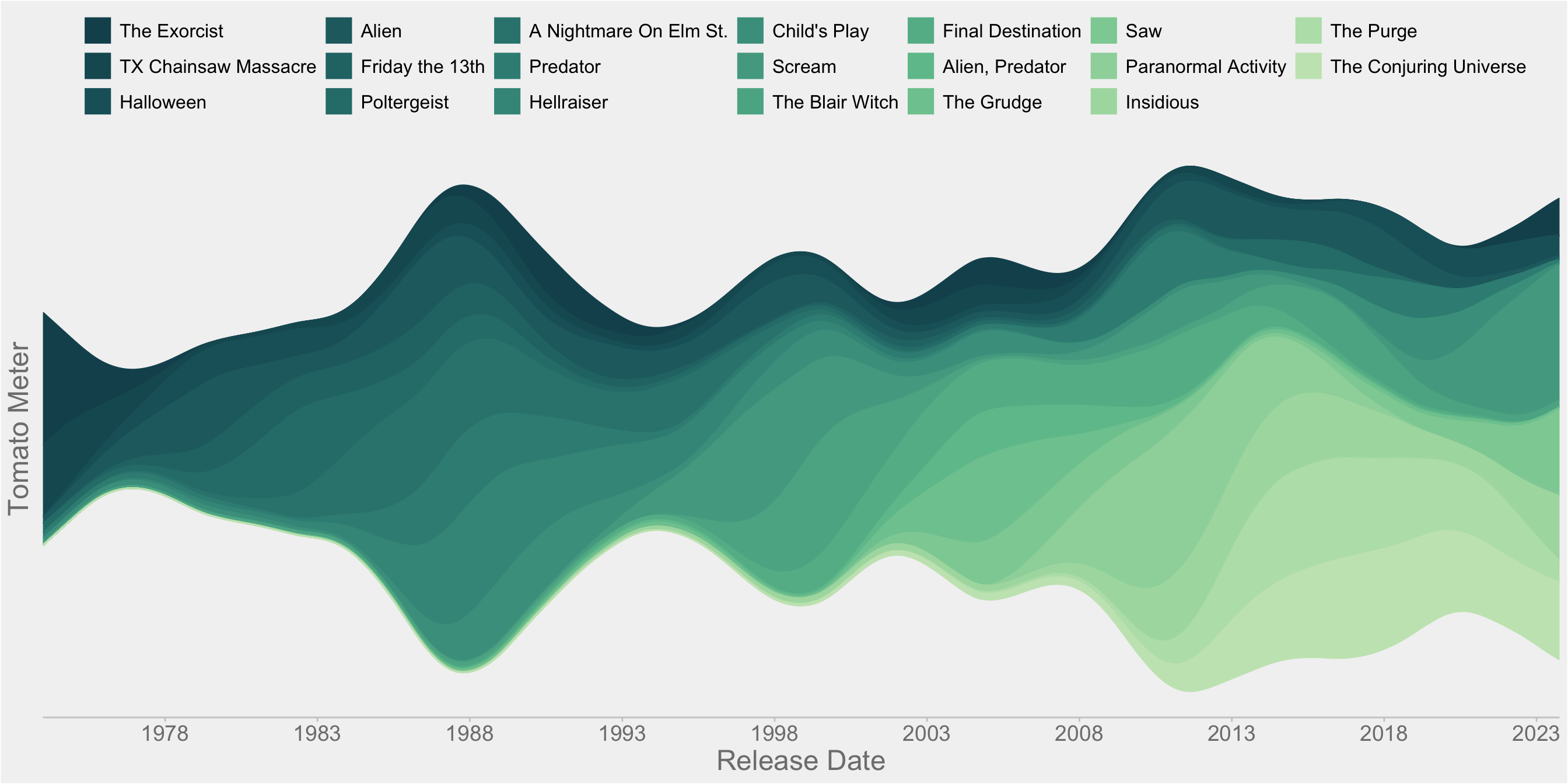
With 20 different levels, the legend can be a bit difficult to visually map onto the stream colors. So, let’s check out geom_stream_label(), which is a nice built in function that adds labels.
Figure 5. Tomatometer score for each franchise over time with labels
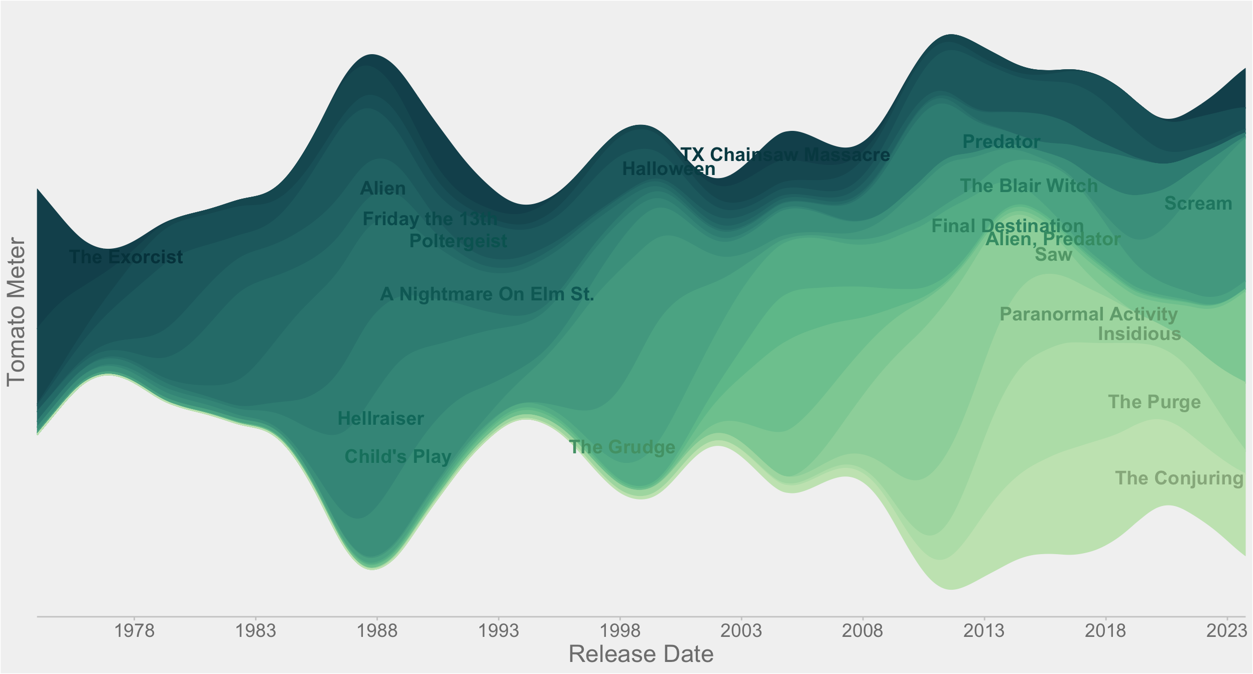
Not too bad – but I found it a bit hard to get the labels where I wanted with this many levels. And I’m not totally sure why the labels are being put where they are.
To try to get a little bit more customization in the labeling, I’m going to use ggplot_build() to get the data that’s generated from the geom_stream_label() call and then modify it. (The reasons I’m calling it after geom_stream_label() is because the transformation into stream-space is done within the geom_stream_label().)
Code to get label data for plot
# Earliest release dataearliest_release <- order_of_release %>%ungroup() %>%rename(label = Franchise)# Get the label dataratings_data <-ggplot_build(ratings_labels)$data[[1]] %>%as_tibble() %>%rename(x0 = x)# Transforming the stream-data back to date datamin_x <-min(ratings_data$x0)target_date <-min(df$`Release Date`)origin_date <- target_date - min_xratings_data$x <-as.Date(ratings_data$x0, origin = origin_date)# Combining the rating data with the earliest release datard <- ratings_data %>%left_join(., earliest_release) %>%mutate(dist_release =abs(x -`Release Date`))# The dates don't line up perfectly, so finding the x values in the label dataset are closest to the initial release date rd <- rd %>%group_by(label) %>%filter(dist_release ==min(dist_release)) %>%# Finding the middle of each streammutate(midpoint =median(y)) %>% dplyr::select(label, x, midpoint) %>%unique()
Code to get label data to add to plot
ratings_repels <- ratings +geom_label_repel(rd,mapping =aes(x = x,y = midpoint,color = label,label = label,fill = label ),inherit.aes = F,segment.color =NA,box.padding =0.35, # Adjust the padding inside the boxpoint.padding =0.5, # Space between the label and the pointmin.segment.length =0,size =5,max.overlaps =11,color ="white" ) +theme(legend.position ="none") +scale_fill_manual(values = pal)ratings_repels
Figure 6
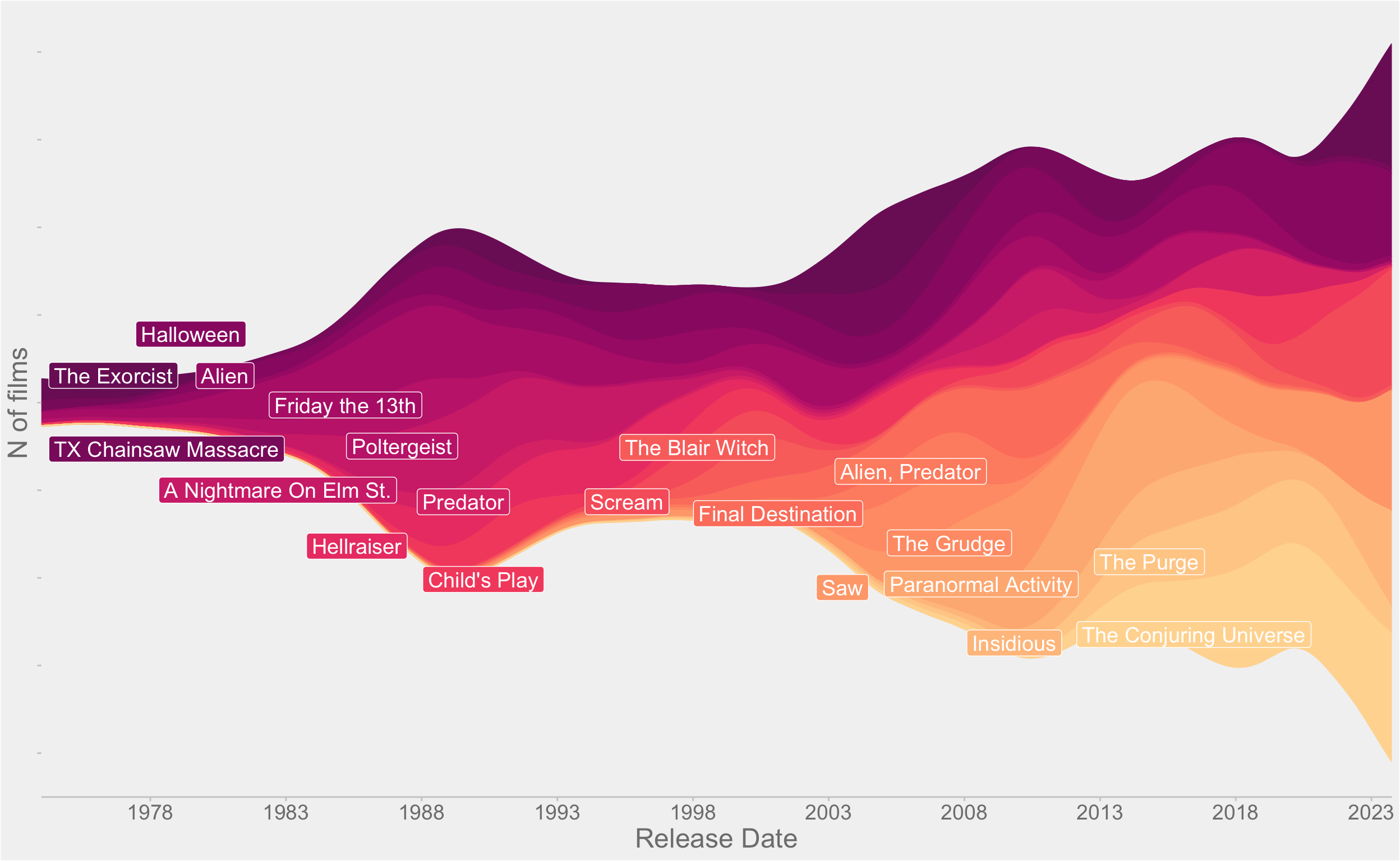
Number of films in each franchise over time
Tomato Meter tells us what Franchise was getting the most ratings when. Let’s switch gears to look at which Franchises dominated the horror market in terms of sheer total number of films over time. We’ll be able to see where Franchises have rapid expansion or stay stable over time.
n_films_repels <- n_films +geom_label_repel(nd,mapping =aes(x = x,y = midpoint,color = label,label = label,fill = label ),inherit.aes = F,segment.color =NA,box.padding =0.35, # Adjust the padding inside the boxpoint.padding =0.5, # Space between the label and the pointmin.segment.length =0,size =5,max.overlaps =11,color ="white" ) +theme(legend.position ="none") +scale_fill_manual(values = pal)n_films_repelsggsave("preview-image.png", n_films_repels,units ="cm", width =32, height =18)
Figure 7. Number of films in each franchise over time with labels
Love to see it. We can see how Nightmare on Elm Street emerging on the market in the late 80s, and Paranormal Activity exploding around the 2010s. And then there’s Child’s Play, consistently releasing films from the late 80s into 2020.
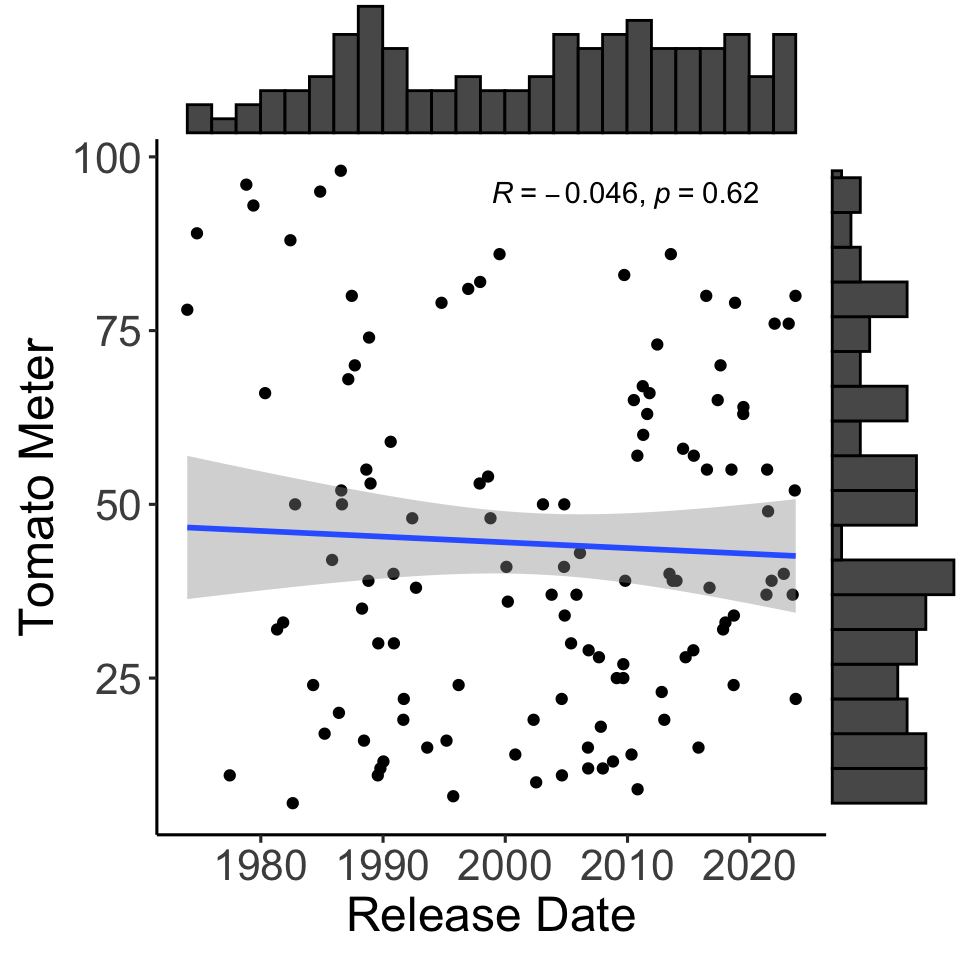
And, just for fun: do ratings change over time?
I was curious to know if there was a general trend in ratings over time – that is, are reviewers generally becoming more or less favorable to horror movies?
Based on Figure 8, looks like no. Looks pretty flat.
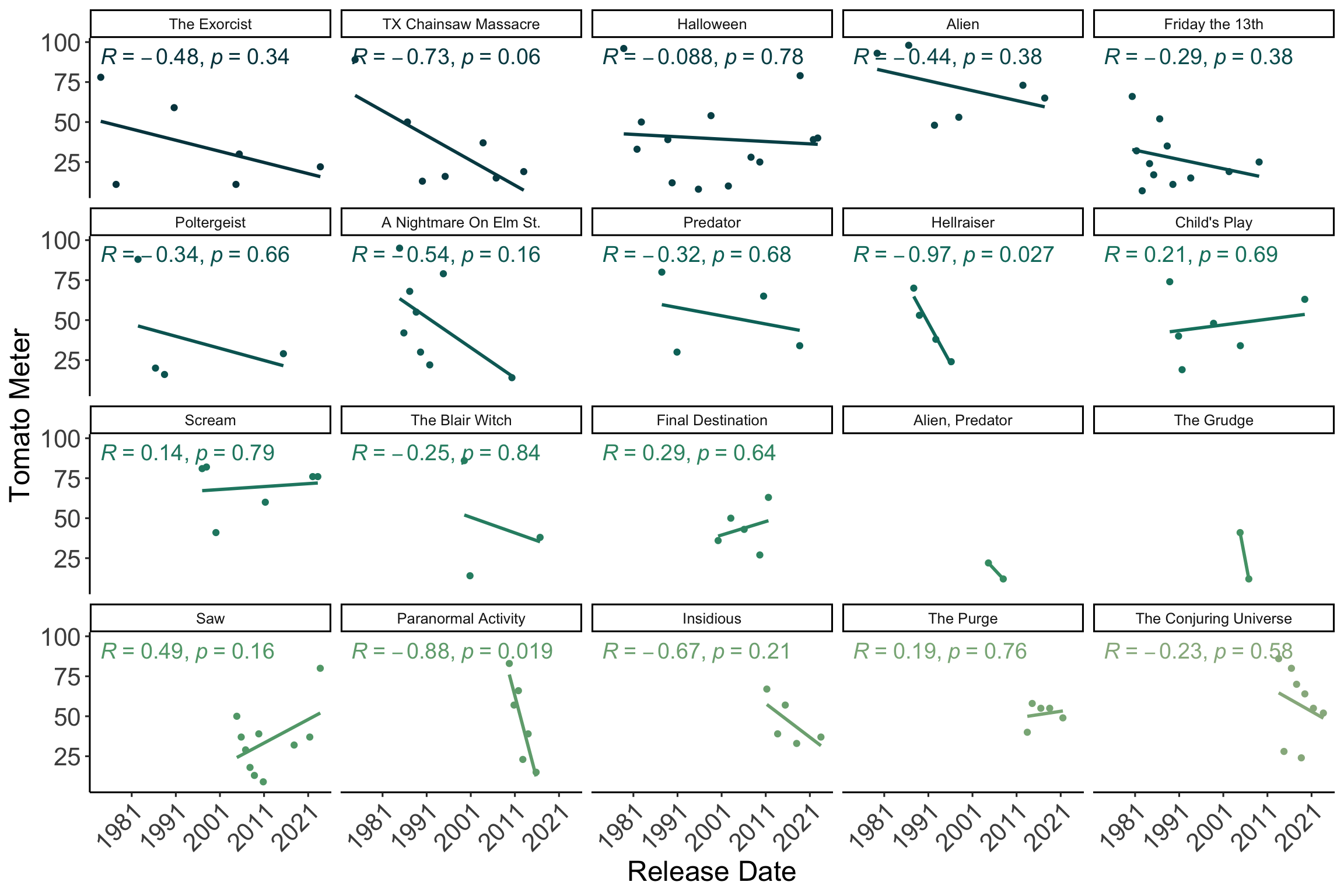
But once you look within Franchises (Figure 9), actually looks like most are showing some trending decrease over time. Specific yikes to Texas Chainsaw Massacre, who has tanked 50 points over it’s 38 years. And Paranormal Activity & Hellraiser, who burned hot and fast, with a 50 point decline over 6-8 years (This dataset doesn’t have the latest Hellraiser…).
Figure 9. Scatterplot of ratings over time for each franchise
Citation
BibTeX citation:
@online{graves2025,
  author = {Graves, Jess},
  title = {Stream Graphs Are a Real Scream 😱},
  date = {2025-02-17},
  url = {https://JessLGraves.github.io/posts/2025-02-13-streamgraph/},
  langid = {en}
}
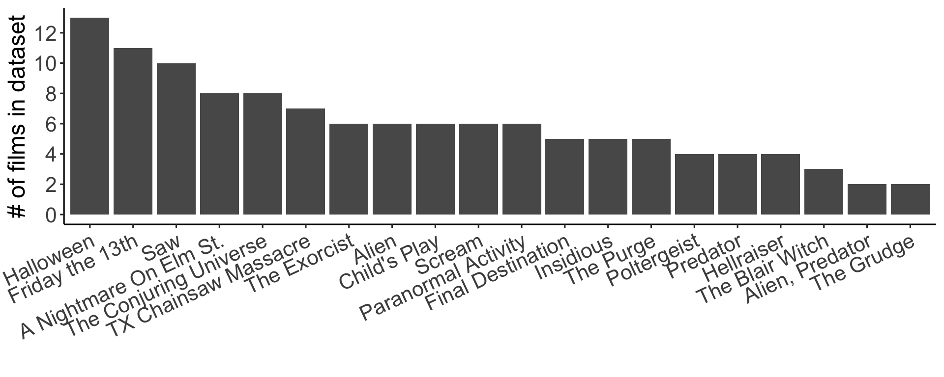
---title: "Stream graphs are a real scream 😱"description: "Looking at horror franchises over time using {ggstream}"author: - name: Jess Gravesdate: 02-17-2025execute-dir: projectcrossref: fig-title: '**Figure**' tbl-title: '**Table**' fig-labels: arabic tbl-labels: arabic title-delim: "."link-citations: trueexecute: echo: true warning: false message: falsecategories: [data visualization, kaggle, blogging-to-learn, R] # self-defined categoriesimage: preview-image.pngdraft: false # bibliography: references.bibnocite: | @*# csl: statistics-in-biosciences.cslbibliographystyle: apacitation: true---## SummaryI recently came across [data-to-viz](https://www.data-to-viz.com/graph/streamgraph.html)'s page on stream graphs and was inspired to learn how to use {[`ggstreams`](https://github.com/davidsjoberg/ggstream)}, [`ggplot_build()`](https://ggplot2.tidyverse.org/reference/ggplot_build.html), {[ggrepel](https://cran.r-project.org/web/packages/ggrepel/vignettes/ggrepel.html)}, and {[`colorspace`](https://colorspace.r-forge.r-project.org)}.## What's a stream graph?From [Wiki](https://en.wikipedia.org/wiki/Streamgraph):Streamgraph: A streamgraph, or stream graph, is a type of [stacked area](https://en.wikipedia.org/wiki/Area_chart) graph which is displaced around a [central axis](https://en.wikipedia.org/wiki/Cartesian_coordinate_system), resulting in a flowing, organic shape.Here is a pretty example that was [made in R](https://r-graph-gallery.com/web-streamchart-with-ggstream.html):[{width="75%"}](https://r-graph-gallery.com/web-streamchart-with-ggstream.html)## Code### Set up libraries & defaults```{r}#| code-summary: Code for libraries & custom functions & themeslibrary(tidyverse)library(lubridate)library(ggstream)library(colorspace)library(patchwork)library(ggrepel)library(ggpubr)library(ggExtra)# setting ggplot thememy_theme <-theme_classic(base_size =12) +theme(axis.title =element_text(size =18),axis.text =element_text(size =16) )theme_set(my_theme)```### The datasetThe data comes from a [kaggle](https://www.kaggle.com/datasets/monkeybusiness7/horror-franchise-box-office-revenues) data set on horror movies. I'm going to be focusing on looking at trends across horror franchises over time.First, a tiny bit of data tidying. I'm going to:1. Get the dates in the right format,2. Drop `Friday the 13th, Nightmare on Elm Street` as a franchise because it's a cross-over with an n of 13. Level the Franchises by their earliest date of release```{r}#| code-fold: falsedf <-read_csv("horror_movie_boxoffice.csv") %>%mutate(`Release Date`=as.Date(`Release Date`, format ="%m/%d/%Y"),Year =year(`Release Date`) ) %>%filter(Franchise !="Friday the 13th, A Nightmare on Elm Street") %>%mutate(Franchise =factor(gsub("The Texas Chainsaw Massacre", "TX Chainsaw Massacre",gsub("Street", "St.", Franchise) )))# Ordering franchises by their earliest release dateorder_of_release <- df %>% dplyr::select(Franchise, `Release Date`) %>%group_by(Franchise) %>%arrange(Franchise, `Release Date`) %>%slice(1) %>%ungroup() %>%arrange(`Release Date`)levels_by_release <- order_of_release$Franchisedf$Franchise <-factor(df$Franchise, levels = levels_by_release)```There are 20 different franchises in this dataset, with Halloween coming in first with the most films in the dataset.```{r}#| label: fig-bar-franchises#| fig-height: 4#| fig-width: 10#| fig-cap: Number of films by franchise franchises <- df %>%group_by(Franchise) %>%tally() %>%arrange(desc(n))franchises %>%mutate(Franchise =factor(Franchise, levels = franchises$Franchise)) %>%ggplot(aes(x = Franchise, y = n)) +geom_bar(stat ="identity") +theme(axis.text.x =element_text(angle =25, hjust =1)) +scale_y_continuous(breaks = scales::pretty_breaks(10)) +labs(x ="", y ="# of films in dataset")```### ggstream()#### Tomato MeterBased on the kaggle documentation, the `Tomato Meter = "The score given by professional critics on Rotten Tomatoes."`I'm going to use `ggstream()` to see what franchises are getting the highest ratings at what point in time.For the sake of illustrating how freaking easy it is to use, I'm going to forgo any formatting for now.```{r}#| label: fig-stream-franchise-nakey#| fig-cap: Boom! One line! geom_stream, you're so easy! #| fig-height: 7#| fig-width: 13#| code-fold: falseratings0 <- df %>%ggplot(aes(x =`Release Date`,y =`Tomato Meter`,fill = Franchise,color = Franchise,text = Franchise,label = Franchise )) +geom_stream()ratings0```Alright, going to try to make it a little more aesthetically pleasing, but using {[colorspace](https://colorspace.r-forge.r-project.org)} to choose my color palette. Because the Franchises are ordered by earliest release date, I'm going to go with a sequential color palette.```{r}#| code-summary: Code for setting paletten_franchise <-length(unique(df$Franchise))# Palette for streamspal <-sequential_hcl(n_franchise, "BluGrn")# Palette for labelspal2 <-darken(sequential_hcl(n_franchise, "BluGrn"), amount =0.2, space ="HCL")``````{r}#| label: fig-palette#| fig-cap: Checking out what my palette will look like #| fig-height: 2#| fig-width: 7#| code-summary: Code for color palette figurecolor_data <-tibble(color =factor(seq_along(pal)),value =1)color_data %>%ggplot(aes(x = color, y = value, fill = color)) +geom_bar(stat ="identity") +scale_fill_manual(values = pal) +theme(legend.position ="none",axis.ticks =element_blank(),axis.text =element_blank(),axis.line =element_blank(),plot.title =element_text(hjust =0.5) ) +labs(x ="", y ="", title ="My custom palette")``````{r}#| code-summary: Code for setting new themenew_theme <-theme_classic() +theme(plot.background =element_rect(fill ="grey95"),panel.background =element_rect(fill ="grey95"),legend.background =element_rect(fill ="grey95"),legend.text =element_text(size =12),axis.line =element_line(color ="grey80"),axis.ticks =element_line(color ="grey80"),axis.text =element_text(color ="grey50", size =14),axis.title =element_text(color ="grey50", size =18),axis.line.y =element_blank(),axis.text.y =element_blank() )theme_set(new_theme)```Time to apply the formatting.```{r}#| label: fig-stream-franchise-2#| fig-cap: Tomatometer score for each franchise over time with formatting#| fig-height: 7#| fig-width: 14#| code-summary: Code for plotratings <- ratings0 +scale_y_continuous(breaks = scales::pretty_breaks(10)) +scale_x_date(breaks ="5 year", date_labels ="%Y",expand =c(0, 0) ) +scale_fill_manual(name ="", values = pal) +scale_color_manual(name ="", values = pal) +theme(legend.position ="top",axis.text.y =element_blank(),axis.ticks.y =element_blank() ) +guides(fill =guide_legend(nrow =3))ratings```With 20 different levels, the legend can be a bit difficult to visually map onto the stream colors. So, let's check out `geom_stream_label()`, which is a nice built in function that adds labels.```{r}#| label: fig-stream-franchise-labels#| fig-cap: Tomatometer score for each franchise over time with labels #| fig-height: 7#| fig-width: 13#| code-fold: falseratings_labels <- ratings +geom_stream_label(fontface ="bold",hjust =0.25,vjust =-0.5,size =5,color = pal2 ) +theme(legend.position ="none")ratings_labels```Not too bad – but I found it a bit hard to get the labels where I wanted with this many levels. And I'm not totally sure why the labels are being put where they are.To try to get a little bit more customization in the labeling, I'm going to use `ggplot_build()` to get the data that's generated from the `geom_stream_label()` call and then modify it. (The reasons I'm calling it after `geom_stream_label()` is because the transformation into stream-space is done within the `geom_stream_label()`.)```{r}#| code-summary: Code to get label data for plot# Earliest release dataearliest_release <- order_of_release %>%ungroup() %>%rename(label = Franchise)# Get the label dataratings_data <-ggplot_build(ratings_labels)$data[[1]] %>%as_tibble() %>%rename(x0 = x)# Transforming the stream-data back to date datamin_x <-min(ratings_data$x0)target_date <-min(df$`Release Date`)origin_date <- target_date - min_xratings_data$x <-as.Date(ratings_data$x0, origin = origin_date)# Combining the rating data with the earliest release datard <- ratings_data %>%left_join(., earliest_release) %>%mutate(dist_release =abs(x -`Release Date`))# The dates don't line up perfectly, so finding the x values in the label dataset are closest to the initial release date rd <- rd %>%group_by(label) %>%filter(dist_release ==min(dist_release)) %>%# Finding the middle of each streammutate(midpoint =median(y)) %>% dplyr::select(label, x, midpoint) %>%unique()``````{r}#| label: fig-streamgragph-repel-labels#| fig-height: 8#| fig-width: 14#| fig-caption: Tomato meter over time with geom_label_repel()#| code-summary: Code to get label data to add to plot ratings_repels <- ratings +geom_label_repel(rd,mapping =aes(x = x,y = midpoint,color = label,label = label,fill = label ),inherit.aes = F,segment.color =NA,box.padding =0.35, # Adjust the padding inside the boxpoint.padding =0.5, # Space between the label and the pointmin.segment.length =0,size =5,max.overlaps =11,color ="white" ) +theme(legend.position ="none") +scale_fill_manual(values = pal)ratings_repels```#### Number of films in each franchise over timeTomato Meter tells us what Franchise was getting the most ratings when. Let's switch gears to look at which Franchises dominated the horror market in terms of sheer total number of films over time. We'll be able to see where Franchises have rapid expansion or stay stable over time.I'm going to pick a different palette for fun.```{r}#| code-summary: Code to set base plot to add labels to# Palettepal <-sequential_hcl(n_franchise, "SunsetDark")n_films <- df %>% dplyr::select(Franchise, `Release Date`) %>%group_by(Franchise) %>%arrange(Franchise, `Release Date`) %>%mutate(`N of films`=row_number()) %>%ggplot(aes(x =`Release Date`,y =`N of films`,fill = Franchise,color = Franchise,label = Franchise )) +geom_stream() +scale_y_continuous(breaks = scales::pretty_breaks(10)) +scale_x_date(breaks ="5 year", date_labels ="%Y",expand =c(0, 0) ) +scale_fill_manual(name ="", values = pal) +scale_color_manual(name ="", values = pal) +theme(legend.position ="none") +guides(fill =guide_legend(nrow =3))``````{r}#| code-summary: Code to get label data # Get the label datans_data <-ggplot_build(n_films)$data[[1]] %>%as_tibble() %>%rename(x0 = x)min_x <-min(ns_data$x0)target_date <-min(df$`Release Date`)origin_date <- target_date - min_xns_data$x <-as.Date(ns_data$x0, origin = origin_date)nd <- ns_data %>%left_join(., earliest_release) %>%mutate(dist_release =abs(x -`Release Date`))nd <- nd %>%group_by(label) %>%filter(dist_release ==min(dist_release)) %>%mutate(midpoint =median(y)) %>% dplyr::select(label, x, midpoint) %>%unique()# # # nd2 <- nd %>%# mutate(# direction = if_else(midpoint < 0,# min(ns_data$y),# max(ns_data$y)# ),# dist_axis = (direction - midpoint),# label_placement = midpoint + dist_axis / .8,# label_placement = if_else(label_placement < 0,# label_placement, -1 * label_placement# )# )``````{r}#| label: fig-stream-franchise-ns#| fig-cap: Number of films in each franchise over time with labels #| fig-height: 8#| fig-width: 13#| code-summary: Code for plotn_films_repels <- n_films +geom_label_repel(nd,mapping =aes(x = x,y = midpoint,color = label,label = label,fill = label ),inherit.aes = F,segment.color =NA,box.padding =0.35, # Adjust the padding inside the boxpoint.padding =0.5, # Space between the label and the pointmin.segment.length =0,size =5,max.overlaps =11,color ="white" ) +theme(legend.position ="none") +scale_fill_manual(values = pal)n_films_repelsggsave("preview-image.png", n_films_repels,units ="cm", width =32, height =18)```Love to see it. We can see how Nightmare on Elm Street emerging on the market in the late 80s, and Paranormal Activity exploding around the 2010s. And then there's Child's Play, consistently releasing films from the late 80s into 2020.## And, just for fun: do ratings change over time?I was curious to know if there was a general trend in ratings over time – that is, are reviewers generally becoming more or less favorable to horror movies?Based on @fig-scatter, looks like no. Looks pretty flat.```{r}#| code-summary: Code for scatter #| label: fig-scatter#| fig-cap: Scatterplot of ratings over time#| fig-width: 5#| fig-height: 5# setting ggplot thememy_theme <-theme_classic(base_size =12) +theme(axis.title =element_text(size =18),axis.text =element_text(size =16) )theme_set(my_theme)p <- df %>% dplyr::select(`Tomato Meter`, Franchise, `Release Date`) %>%ggplot(aes(x =`Release Date`, y =`Tomato Meter`)) +geom_point() +theme(legend.position ="none") +stat_smooth(method ="lm") +stat_cor(label.y.npc ="top",label.x.npc ="center" )ggMarginal(p,type ="histogram",xparams =list(binwidth =365*2),yparams =list(binwidth =5))```But once you look within Franchises (@fig-scatter-by-franchise), actually looks like most are showing some trending decrease over time. Specific yikes to Texas Chainsaw Massacre, who has tanked 50 points over it's 38 years. And Paranormal Activity & Hellraiser, who burned hot and fast, with a 50 point decline over 6-8 years (This dataset doesn't have the latest Hellraiser...).```{r}#| code-summary: Code for scatter with correlations#| label: fig-scatter-by-franchise#| fig-cap: Scatterplot of ratings over time for each franchise#| fig-width: 12#| fig-height: 8df %>% dplyr::select(`Tomato Meter`, Franchise, `Release Date`) %>%ggplot(aes(x =`Release Date`, y =`Tomato Meter`,color = Franchise, fill = Franchise )) +geom_point() +theme(legend.position ="none",axis.text.x =element_text(angle =45, hjust =1) ) +stat_smooth(method ="lm", se = F) +scale_fill_manual(values = pal) +scale_color_manual(values = pal2) +stat_cor(label.x.npc ="left", label.y =90,size =5 ) +facet_wrap(~Franchise) +scale_x_date(date_labels ="%Y", breaks ="10 year")```